The December 2022 release of Power BI Desktop includes three new DAX functions: OFFSET, INDEX, and WINDOW. They are collectively called window functions because they are closely related to SQL window functions, a powerful feature of the SQL language that allows users to perform calculations on a set of rows that are related to the current row. Because these functions are often used for data analysis, they are sometimes called analytical functions. In contrast, DAX, a language invented specifically for data analysis, had been missing similar functionalities. As a result, users found it hard to write cross-row calculations, such as calculating the difference of the values of a column between two rows or the moving average of the values of a column over a set of rows. Oftentimes even if there is a way to perform such calculations, the resulting expressions are convoluted and cause DAX Engine to consume too much time and memory, therefore, don’t scale to larger number of data points. For these reasons, the DAX product team is super-excited to present the first batch of window functions as an early Christmas gift to the DAX community. Like their SQL counterparts, the DAX window functions are powerful yet more complex than most other DAX functions therefore require more effort to learn. In this blogpost, I’ll describe the syntax and semantics of these functions with a couple of concrete examples so that you can have the correct mental model when you work with these functions. In my next blogpost, I’ll dive deeper under the cover to expose some of the inner workings of the these functions to help you design your own solutions with good performance.
All examples will be based on the Adventure Works DW 2020 DAX sample model.
A TASTE OF DAX WINDOW FUNCTIONS
Let’s jump right in and create the first report using the OFFSET function.
- First add columns ‘Customer'[Customer], ‘Date'[Date], and measure [Total Quantity] to a simple table report.
- Next apply a filter to limit the rows to customers with multiple sales dates.
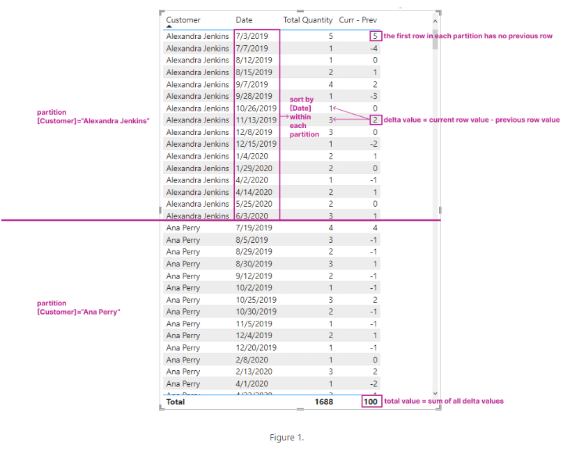
- Now come the interesting part: define a measure [Curr – Prev] that, for each customer and sales date, calculates the delta of [Total Quantity] between the current sales date and the previous sales date.
- Add [Curr – Prev] to the table to see the result in Figure 1.
- It can be easily seen that the delta values are all correct. I have also verified that the total value, 100, is the sum of all the delta values.
Curr - Prev =
    [Total Quantity] -
    CALCULATE(
        [Total Quantity],
        OFFSET(
            -1,
            SUMMARIZE(ALLSELECTED('Sales'), Customer[Customer], 'Date'[Date]),
            ORDERBY('Date'[Date]),
            KEEP,
            PARTITIONBY(Customer[Customer])
        )
    )
ADVANTAGES OF THE WINDOW FUNCTIONS
When the OFFSET function was first leaked a couple of months ago, some users questioned its usefulness. They argued that they could achieve the same results using existing DAX functions such as time intelligence functions or setting appropriate filters in the CALCULATE function in the following fashion:
CALCULATE(
    ...,
    VAR Curr = VALUES([OrderByColumn])
    RETURN
    FILTER(ALL([OrderByColumn]), [OrderByColumn]=Curr-1)
)
But window functions are more generic and powerful in that
- The order-by values don’t need to be continuous.
- Users can order by multiple columns, e.g. first by [Year] and then by [MonthNumberOfYear].
- Users can divide rows of a table into partitions and then sort the rows in each partition independently. You can see from our first example that the [Date] values are different in the two partitions in Figure 1.
- Window functions offer simpler, consistent syntax and better performance than previous solutions using the FILTER function. For those who have studied computer science, the difference in time and space complexity is O(N*Log(N)) or even O(N) for window functions vs O(N2) for hand-crafted FILTER expressions.
SYNTAX OF WINDOW FUNCTIONS
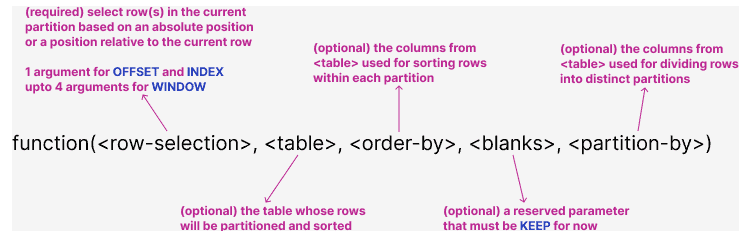
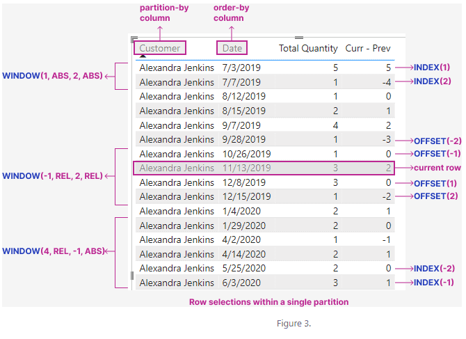
Although each window function has its own unique signature, they all follow the same pattern and share common parameters as shown in Figure 2. <row-selection> is the only required parameter(s) that defines the unique characteristics of each function. See Figure 3 for the different ways to select rows from a partition.
Any function that takes more than a couple of input parameters appear daunting to the users. For that reason, window functions may look too complex to beginners. But the good news is that most of the parameters are optional. Moreover, the DAX product team has made all optional parameters skippable even if they are not the last parameter. As long as you don’t mind some red-squiggly in the Desktop formula bar, the following DAX expressions are all accepted by the DAX Engine.
Some of the shortcut syntaxes are not yet accepted in the formula bar, therefore you will see the red-squiggly underneath, but they are valid according to DAX Engine. More work is planned for them to be accepted by the formula bar in a future release.
| The KEEP keyword in between <order-by> and <partition-by> can be omitted. e.g. OFFSET(-1, ALLSELECTED(‘Date’), ORDERBY([Date]), PARTITIONBY([Fiscal Year])) |
| <table> can be omitted if <order-by> is present. In this case all columns in <order-by> and <partition-by> must belong to the same table. e.g. INDEX(1, ORDERBY(‘Date'[Date]), PARTITIONBY(‘Date'[Fiscal Year])) |
| <order-by> can be omitted. In this case DAX Engine will automatically inject order-by columns. e.g. WINDOW(2, ABS, -2, ABS, ALL(‘Date’), PARTITIONBY([Fiscal Year])) |
| <from-type> and <to-type> can be omitted in the WINDOW function. In this case the type is defaulted to REL. The formula bar already supports skipping these parameters completely. e.g. WINDOW(-3, -1, ALL(‘Date’)) |
Shortcut syntaxes
HOW DO WINDOW FUNCTIONS WORK
The list below describes the logical steps performed by each window function:
- Take all rows of the table as specified by the <table> parameter.
- Divide the rows into separate partitions by the unique values of the partition-by columns.
- Sort the rows within each partition according to the order-by columns and sorting directions.
- Determine the current partition and, if necessary, the current row within the partition.
- Return zero, one or more rows within the current partition.
- OFFSET returns 0 or 1 row at a certain distance from the current row.
- INDEX returns 0 or 1 row at a fixed position in the current partition.
- WINDOW returns all the rows in between a lower bound and an upper bound. Either bound is a row at a certain distance from the current row or at a fixed position in the current partition.
In addition to the general rules listed above, there are some special, yet common use cases, which are worth calling out:
- When the <table> parameter is omitted, DAX Engine derives the table expression from the order-by and partition-by columns as ALLSELECTED(<order-by columns>, <partition-by columns>). In this case all columns must be from the same table.
- When the <partition-by> parameter is omitted, the entire table is treated as a single partition.
- When the <order-by> parameter is omitted, DAX Engine will order by all the columns in the table. This is convenient when there is only a single column in the table, but not recommended when there are more than one column, in which case it’s a good practice to explicitly specify the order-by columns so the sort order is fully controlled by the user.
- When the user-specified order-by columns are insufficient to determine the order of all the rows, i.e. there can be ties among some rows, DAX Engine will automatically append additional order-by columns from the table until total order is achieved. If this is not possible because the table has no key columns therefore there maybe duplicate rows, DAX Engine will return an error. Users should always provide enough order-by columns to achieve total order if they want to have full control.
HOW IS THE CURRENT PARTITION OR THE CURRENT ROW DETERMINED
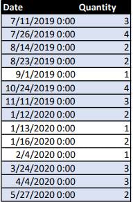
Since all window functions depend on the current partition and/or the current row to work properly, how do they know what the current partition or the current row is? In comparison, a SQL query always scans a set of rows in the FROM clause so the current row is natural for SQL window functions. On the DAX side, iteration functions such as SUMX, FILTER, SELECTCOLUMNS, GENERATE, etc. also work one row at a time, a window function could leverage that to determine the current partition and current row. For example, when I was writing this blog, someone asked how to filter a given table of sales over dates to keep only those rows with consecutive sales above a threshold. This is a very typical business problem for window functions to solve. If we extract one partition, corresponding to ‘Customer'[Customer] = “Antonio Bennett”, from the table in Figure 1, we get the table in Figure 4. If we want to find out consecutive rows where [Quantity] >= 2, i.e. the highlighted rows, we could use the following DAX query to achieve the result:
DEFINE
VAR _Table =
    SUMMARIZECOLUMNS(
        'Date'[Date],
        TREATAS({"Antonio Bennett"}, 'Customer'[Customer]),
        "Quantity", [Total Quantity]
    )
EVALUATE
    FILTER(
        _Table,
        [Quantity] >= 2 &&
        (
            SELECTCOLUMNS(OFFSET(-1, _Table, ORDERBY([Date])), [Quantity]) >= 2 ||
            SELECTCOLUMNS(OFFSET(1, _Table, ORDERBY([Date])), [Quantity]) >= 2)
        )
ORDER BY [Date]
In the DAX query above, both the FILTER function and the two OFFSET functions scan the rows from the same table variable, _Table, so it’s pretty easy to see that the two OFFSET functions would use the current row added by FILTER to the row context. In general, there is an evaluation context when a window function is calculated, so the window function will derive the current partition and the current row from its evaluation context.
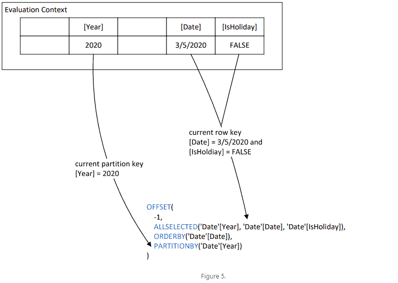
To determine the current partition, a window function would look for the partition-by columns from row context or from the grouping columns in the filter context. If a match is found, it will use the values of those columns in the context as the key for the partition.
Similarly to determining the current row, a window function would use the same strategy but this time checking for all columns from the <table> parameter. To be precise, only model columns from <table> are considered because only model columns can be added to the filter context.

Is it possible for a current row from the context to not have a match to a row from the <table>? Absolutely, the rows from the outer context and the rows from the <table> parameter of a window function are independent of each other in the general case. There can be more rows in the context than rows from the inner table, or vice versa. This is very different from SQL window functions which are tightly coupled with the main query.
WHAT IF THERE IS NO CURRENT PARTITION OR CURRENT ROW
In the previous example, we are lucky in that the evaluation context happens to have all columns necessary to identify the current row. But what if some columns are missing, or, worse yet, all columns are absent? DAX expressions must work in all contexts, that’s the fundamental reason that measures can be reused in any report. The DAX engine team has implemented a concept, called apply semantics, to window functions so that they not only don’t fail when there isn’t enough information in the evaluation context to identify a unique partition or row but they even return meaningful results in common scenarios. The name, apply semantics, was inspired by the CROSS APPLY operator of T-SQL.
Below is the logic of the apply semantics assuming a window function requires the current row:
- Divide all columns from <table> into those that can bind to the evaluation context and those that cannot.
- Build an iterator to return rows from the outer context corresponding to the bound columns in #1.
- For each row R1 from #2, build an iterator to return all possible rows corresponding to the unbound columns in #1 that exists with the R1. For example, if [Column] is the only unbound column, iterate over all rows returned by VALUES([Column]).
- For each row R2 from #3, combine R1 and R2 into R. R has values for all columns in #1, therefore is a valid current row.
- Use R to locate the current partition and then the current row within the partition.
- Calculate the result row(s) as defined by the semantics of the window function.
- Output the row(s) as long as it has not been output already.
As you can see, apply semantics effectively enumerates all valid current partitions/rows in a given context, calculates the regular output of a window function for each partition/row, and then returns the union of the output without duplicates. As a result, OFFSET and INDEX may return more than one row, and WINDOW may return more rows than the size of the window. Going back to Figure 1, in order to calculate the value of [Prev – Curr] in the grand total row, DAX Engine iterates over all valid combinations of [Customer] and [Date], shifts to the previous [Date] value within the given [Customer] partition, and in the end outputs all rows in the table except for the last rows in each partition and then use that as a filter to calculate the difference between the values of measure [Total Quantity] with and without the filter.
The apply semantics poses a potential performance risk when the unbound columns come from different dimension tables therefore may produce a big cross-join in contexts without sufficient filters. DAX authors should pay close attention if they use window functions in this fashion.
SUMMARY
The advent of window functions in DAX opens a floodgate of opportunities for Power BI users to solve complex, even previously intractable, problems in an efficient, uniform, and elegant way. They can be used to perform a wide range of calculations on sets of data, e.g.
- Compute running totals and running averages
- Find best and worst performers
- Investigate trends across time
- Calculate contributions to the whole, such as commission percentages
Moreover, this is just the initial release with limitations and known issues. The DAX product team is actively working on additional improvements and new features to enrich this category of functions so users can expect more exciting capabilities to arrive in the near future.
This blog is part of Power Platform Week.
About the Author
Partner Architect at Microsoft
Reference
Wang, J., 2022, INTRODUCING DAX WINDOW FUNCTIONS (PART 1), Available at: Introducing DAX Window Functions (Part 1) – pbidax (wordpress.com) [Accessed on 18 January 2023]