This is the second installment in our two-part series on DAX window functions announced in the December 2022 release of Power BI Desktop. I will first answer the questions that I had received from the community about topics covered in the first article, and then go into more technical details about the implementations of these functions to help advanced users understand the performance characteristics of these functions when working with large volumes of data.
Just like last time, all examples will be based on the Adventure Works DW 2020 DAX sample model. The final pbix file that includes all DAX expressions used for this blog post can be downloaded from here.
THE TABLE TO BE SORTED CANNOT HAVE DUPLICATE ROWS
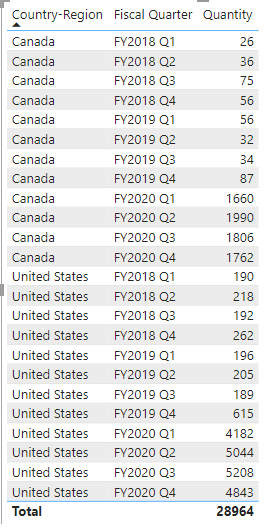
Several people had reported running into errors when trying the window functions on fact tables. Let’s look at an example by first adding a calculated table of three columns to the model that is defined by the following DAX expression, and then, add all three columns to a table visual as shown in Figure 1.
CalcTable = SUMMARIZECOLUMNS(
    'Customer'[Country-Region],
    'Date'[Fiscal Quarter],
    TREATAS({"Canada", "United States"}, 'Customer'[Country-Region]),
    "Quantity", [Total Quantity]
)
Next we want to create a measure to return the [Quantity] value in the previous row. However, if you define the measure using the DAX expression below you’ll get the error in Figure 2 that the relation parameter, ALLSELECTED(‘CalcTable’), may have duplicate rows.
Prev Qtr = CALCULATE(
    SUM(CalcTable[Quantity]),
    OFFSET(
        -1,
        ALLSELECTED('CalcTable'),
        ORDERBY([Fiscal Quarter]),
        PARTITIONBY([Country-Region])
    )
)

Two questions immediately come to mind:
- What can go wrong if the <table> parameter had duplicate rows?
- Since ‘CalcTable’ clearly has no duplicate rows, why did we get the error in the first place?
To answer the first question, please note that all window functions rely on sorted rows in each partition to determine the absolute or relative positions of the current row and the corresponding output row(s). If the table had duplicate rows, what would be the position numbers assigned to tied rows? Even if the DAX Engine assigns continuous position numbers to a set of tied rows, when the current row from the context matches the tied rows, which position number should the DAX Engine pick? One may argue that although the error is understandable if a current row is required, how come the INDEX function still raises the error even though it does not require a current row to determine its output row? Let us image a scenario where the index number points to one of the tied rows. Should the DAX Engine return just one row, or all the tied rows like what the TOPN function does? Due to these potential ambiguities, the DAX Engine does not allow duplicate rows in the table to be sorted, therefore, it needs a way to find out whether a table may have the problem.
Although the DAX Engine can analyze a DAX table expression to determine whether it has duplicate rows, it relies on metadata saved in the model to find out whether a model table, including calculated tables, has duplicate rows. That means all dimension tables do not have duplicate rows because they must have a primary key column as the endpoint of a relationship. But fact tables, or any standalone tables, are treated as potentially having duplicate rows. The DAX Engine does not attempt to detect row uniqueness at runtime because that may change after the next data refresh. Since our example truly has no duplicate rows and the underlying table is quite small, we could use the DISTINCT function as a workaround to inform the DAX Engine of no duplicate rows at the cost of performance overhead.
Prev Qtr = CALCULATE(
    SUM(CalcTable[Quantity]),
    OFFSET(
        -1,
        DISTINCT(ALLSELECTED('CalcTable')),
        ORDERBY([Fiscal Quarter]),
        PARTITIONBY([Country-Region])
    )
)
AVOID CIRCULAR DEPENDENCY ERROR IN CALCULATED COLUMNS
Last time, we said that the DAX Engine uses all the columns from the <table> parameter to determine the current partition and the current row. This semantics poses a special challenge when using the window functions to define calculated columns. That is because one of the most natural ways to specify the <table> parameter in a calculated column expression is simply using the hosting table name. For example, if I were to add a column to the ‘Customer’ table to return the previous customer within the same city, I could use the following expression.
Prev Customer = SELECTCOLUMNS(
    OFFSET(-1,
        'Customer',
        ORDERBY([Customer ID]),
        PARTITIONBY([City])
    ),
    [Customer]
)
It’s a calculated column expression, not a measure expression.
I used a shortcut syntax of the SELECTCOLUMNS function not yet supported by the formula bar so you will see a red squiggly line under [Customer] if you try the expression yourself but it is accepted by the DAX Engine.
Currently, the expression is accepted by the Desktop due to a product defect but may cause an error in the service where the bug fix has already been deployed or will be deployed soon. The problem is that the table reference ‘Customer’ includes all columns in the table. Since window functions are supposed to use all columns to calculate the current row, the values of the calculated column expression depends on the values of all columns of ‘Customer’, including itself, hence a circular dependency error! Even if the DAX Engine removes the current calculated column from consideration, so that only the rest of the columns from the table are taken into account, we will quickly run into circular dependency again if we were to add a second calculated column such as [Next Customer] because [Prev Customer] depends on all other columns including [Next Customer] while the latter depends on all other columns including the former. Before the product team introduces a less verbose option, it’s recommended that all calculated columns use the SELECTCOLUMNS function to explicitly list all the columns from the hosting table needed for the calculation. So we should modify the DAX expression of [Prev Customer] by using the shortcut version of SELECTCOLUMNS again:
Prev Customer = SELECTCOLUMNS(
    OFFSET(-1,
        SELECTCOLUMNS('Customer', [CustomerKey], [Customer ID], [City], [Customer]),
        ORDERBY([Customer ID]),
        PARTITIONBY([City])
    ),
    [Customer]
)
You must always include the key column of the dimension table, [CustomerKey] in this case, to satisfy the no duplicate row requirement as described in the previous section.
A MORE ACCURATE DESCRIPTION OF THE APPLY SEMANTICS

- Find all possible rows of columns from <table> by taking into account the current evaluation context, e.g. apply all filters.
- For each row from #1, locate the current partition and then the current row within the partition, perform steps #3 and #4.
- Calculate the result row(s) as defined by the semantics of the window function.
- Output the row(s) as long as they have not been output already.
DEBUG WINDOW FUNCTIONS BY PRINTING INTERMEDIATE RESULTS
Window functions are among the more complex table functions. In the past, it is usually hard to figure out what goes wrong when a formula containing a table function doesn’t return expected results. Luckily, three new DAX functions, EVALUATEANDLOG, TOCSV, TOJSON, were released just in time to make it very easy to see the output of any table expression. For example, if I were to use the above DAX expression as is, without wrapping ‘Customer’ in ALLSELECTED, to create a measure instead of a calculated column, I would get an empty visual if I added the measure to a table visual, with the total row turned off, alongside columns [City], [Customer ID], and [Customer]. Using two EVALUATEANDLOG functions to inspect both the input and the output of the OFFSET function, I can see, in DAX Debug Output, the empty outputs of the OFFSET function, Figure 3, and many single row tables, one per input row, as the input to OFFSET, Figure 4. The bug lies in the fact that OFFSET, in our case, is supposed to partition and sort the same static table independent of the input rows, but instead, the table expression is filtered by them therefore produces a different table for each input row. It’s a very big topic to understand how to interpret the output of the EVALUATEANDLOG function. If you are interested, see my previous blog posts, 1, 2, 3, 4.


IMPLEMENTATION DETAILS THAT MAY AFFECT PERFORMANCE
You can skip the rest of the article unless you need to pass a large number of rows, e.g. more than a couple of millions, to the window functions. For the advanced users who are aware of the division of labor between the formula engine and the storage engine, DAX window functions are implemented strictly inside the formula engine. That means window functions are not pushed into the Vertipaq Engine for import models or folded into SQL for DirectQuery models. The rationale for this design decision was based on the observation that window functions are typically applied on top of aggregated values instead of to the raw data in the fact tables.
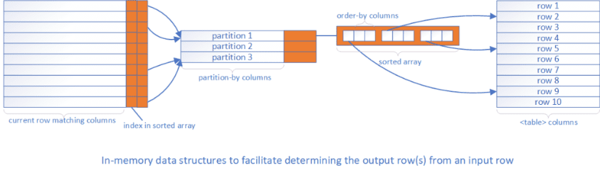
One consequence of implementing all window functions in the formula engine is that the formula engine must have a copy of all the rows of the input table. Even if the input table is an imported table, the formula engine still makes a copy of the table rows into its own spool structure instead of reusing the data in the Vertipaq Engine. Moreover, the formula engine creates additional in-memory data structures to facilitate fast mappings from any current row as determined by the context to output rows of the <table> parameter. Figure 5 depicts the in-memory data structures created by the formula engine to implement a window function that takes an input row from the context to calculate output row(s) from a static table. The diagram consists of three spools:
- The rightmost spool stores the raw data from the static table.
- The middle spool maps partition-by columns to sorted arrays. Each array stores sorted rows within a partition.
- The leftmost spool maps matching columns to the corresponding partition and the index of the row in the sorted array.
Although Figure 5 is just one example, all window functions are implemented following a similar pattern with more or less memory used as required by the semantics of the specific function. As one could imagine, the memory overhead can be quite significant when there are many columns and rows in the <table> therefore users should strive to minimize both to reduce memory consumption.
CONCLUSION
DAX window functions have generated a lot of excitement because they enable users to define calculations over a set of rows related to the current row. Even though they are released during the holiday season, the DAX community has already provided valuable feedbacks for the product team to further refine and enrich the design and functionality. DAX developers can expect to see continuous improvements to these functions in the upcoming new year.
This blog is a part of Power Platform Week.
About the Author
Partner Architect at Microsoft
Reference
Wang, J., 2022, INTRODUCING DAX WINDOW FUNCTIONS (PART 2), Available at: INTRODUCING DAX WINDOW FUNCTIONS (PART 2) – pbidax (wordpress.com) [Accessed on 18 January 2023]